Everything about FFNs: Structure, Optimization and Beyond

Mathematical formulation

A standard fully-connected neural network is given by

\[f_\theta(x) = W^L\phi(W^{L-1}\cdots \phi(W^2\phi(W^1x)))\]

where $\phi: \mathbb{R} \rightarrow \mathbb{R}$ is the neuron activation function, $W^l$ is a matrix of dimension $d_j \times d_{j-1}, l=1, \cdots, L$ and $\theta = (W^1,\cdots,W^L)$ represents the colelction of all parameters. When applying the scalar function $\phi$ to a matrix $Z$, we apply $\phi$ to each entry of $Z$. Another way to write down the neural network is to use a recursion formula

\[z^0 = x, z^l = \phi(W^l z^{l-1}+ b^l), l= 1,\cdots L.\]

For simplicity of presentation, we skip the bias term $b^l$ in the expression of neural networks. For computer vision tasks, convolutional neural networks (CNN) are standard. For an input $Z$ of size $I \times I \times C$, where $C$ is the number of channels, A filter $W$ of size $F \times F \times C$ produce an output of size $O \times O \times 1$. The indexes of rows and columns of the result matrix are marked with $m$ and $n$ respectively.

\[Z^l(m,n) = (Z^{l-1} * W^{l}) (m,n) = \sum_{i=1}^F\sum_{j=1}^F\sum_{k=1}^C W^l(i,j,k) Z^{l-1}(m+i-1,n+j-1,k).\]

Please be noted this definition is different from mathmetical definition of convolusion of two funcitons, where the place of $+$ and $-$ should be switched. If there is an application of $K$ filters, it will result in an output of size $O \times O \times K$. If there is a stride $S$, then the convulution index on the input becomes $Z^{l-1}(m +(m-1)s+i-1, n+(n-1)s+j-1,k)$.

The pooling layer (POOL) is a downsampling operation, typically applied after a convolution layer, which does some spatial invariance. The operation is similar to convolution, but instead of weighted sum, it is replaced with maximum or average.

Zero-padding denotes the process of adding P zeroes to each side of the boundaries of the input. There are three types of padding. $P = 0$ denotes the valid padding. $P_s = \lfloor\frac{S\lceil\frac{I}{S}\rceil - I + F - S}{2}\rfloor$ and $P_e = \lceil\frac{S\lceil\frac{I}{S}\rceil - I + F - S}{2}\rceil$ are called the same padding, such that ouput has size $\lceil\frac{I}{S}\rceil$. $P_s \in [0,F-1]$ and $P_e = F-1$ are called the full padding. Finally, the output size $O$ is given by

\[O = \frac{I - F + P_s + P_e}{S} + 1.\]

The last type of neural networks we mention in this article is Residual Network (ResNet). A nested sequence of function classes $\mathcal{F}_ 1 \subseteq \cdots \subseteq \mathcal{F}_ L$ will enhance its capability of finding the optimum. Therefore, we would require the mapping between two layers ($\mathcal{F}_ {l-1}$ and $\mathcal{F}_ l$) includes the identity map $\mathcal{H}(x) = x$, or the residual map $\mathcal{F}(x) = \mathcal{H}(x) - x$. The original function thus becomes $\mathcal{F}(x) + x$. The building blocks of ResNet look like

\[z^l = \phi(\mathcal{F}(z^{l-k},\{W^{j}\}_ {j=l-k}^l) + z^{l-k}),\]

where $\mathcal{F}$ repressents the residual mapping to be learned, For example, two layers, $\mathcal{F}(z^{l-1}) = W^l\phi(W^{l-1}z^{l-1})$.

Backpropagation

From an optimization perspective, backpropagation is an efficient implementation of gradient computation. To illustrate how BP works, suppose the loss function is quadratic and consider the per-sample loss

\(F(\theta) = \|y - W^L\phi(W^{L-1} \cdots W^2\phi(W^1x))\|^2\).

We define an important set of intermediate variables

\(z^0 = x, h^1 = W^1 z^0,\) \(z^1 = \phi(h^1), h^2 = W^2 z^1,\) \(\cdots\) \(z^{L-1} = \phi(h^{L-1}), h^L = W^L z^{L-1}.\)

Furthermore, define $D^l = diag(\phi’(h_1^l),\cdots, \phi’(h_d^l))$, which is a diagonal matrix with the $i$-th diagonal entry being the derivative of the activation function evaluated at the $i$-th pre-activation $h_i^l$. Let the error vector $e = (h^L - y)^2$. The gradient over weight matrix $W^l$ is given by

\[\frac{\partial F(\theta)}{\partial W^l} = -(W^LD^{L-1} \cdots W^{l+1}D^l)^\top 2(h^L - y)(z^{l-1})^\top, l = 1,\cdots, L.\]

Define a sequence of backpropagated error as

\(e^L = 2(h^L - y),\) \(e^{L-1} = (D^{L-1}W^L)^\top e^L,\) \(\cdots\) \(e^1 = (D^1W^2)^\top e^2.\)

Then the partial gradient can be written as

\[\frac{\partial F(\theta)}{\partial W^l} = -e^l(z^{l-1})^\top, l = 1,\cdots, L.\]

A naive method to compute all partial gradients would require $\mathcal{O}(L^2)$ matrix multiplications since each partial gradients requires $\mathcal{O}(L)$ matrix multiplication. A smarter algorithm is to reuse multiplications as follow.

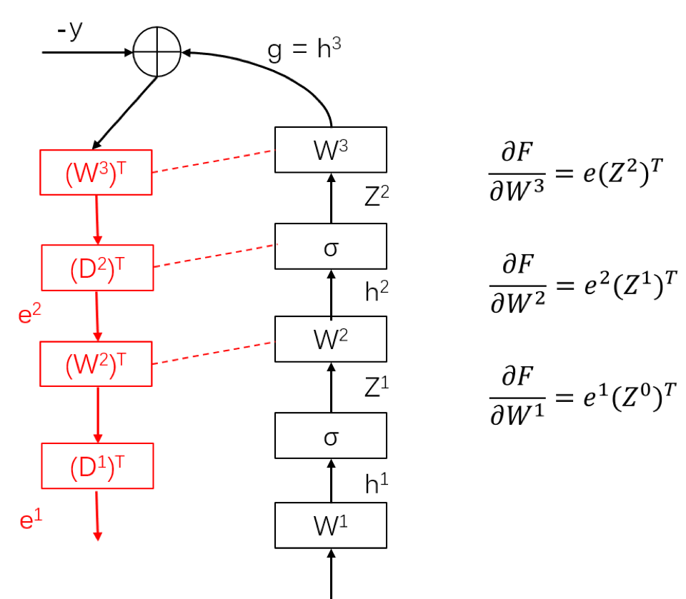
In the forward pass, from the bottom layer $1$ to the top layer $L$, post-activation $z^l$ is computed recursively and stored for future use. After computing the last layer ouput $h^L$, we compare it with the ground-truth $y$ to obtain the error $e = (h^L - y)^2$. In the backward pass, from the top layer $L$ to the bottom layer $1$, two quantities are compared at each layer $l$. First, the backpropagated error $e^l$ is computed. Second, the partial gradient over the $l$-th layer weight matrix $W^l$ is computed. After the forward pass and backward pass, we have computed the partial gradient for each weight for one sample $x$.

By a small modification to this procedure, we can implement SGD as follows. After tge partial gradient over $W^l$ is computed, we update $W^l$ by a gradient step. After updating all weights $W^l$, we have completed one iteration of SGD. In mini-batch SGD, the implementation is slightly different: in the feedforward and backward pass, a mini-batch of multiple samples will pass the network together.

Gradient Explosion / Vanishing

Consider the following example of $1$-dimensional problem

\[\min_{w_1,\cdots,w^L} F(\theta) = (1 - w^1\cdots w^L)^2.\]

The gradient over $w^l$ is

\[\frac{\partial F(\theta)}{\partial w^l} = -2w^1\cdots w^{l-1}w^{l+1}\cdots w^L(1-w^1\cdots w^L) = -2w^1\cdots w^{l-1}w^{l+1}\cdots w^L e.\]

If all $w^l = 2$, then thegradient has norm $2^{L-1}e$ which is exponentially large, if all $w_l = \frac{1}{2}$, then the gradient has norm $(\frac{1}{2})^{L-1}e$ which is exponentially small. Note that many works do not mention gradient explosion, but just mention gradient vanishing. This is partially because the non-linear activation function can reduce the signal, partially because empirical tricks such as gradient clipping and partially because regularization.

ReLu Activation

The use of sigmoid type of activation functions, such as logistic sigmoid function $\phi(x) = \frac{1}{1+\exp(x)}$, suffers from gradient vanishing problem. Recall the backpropagated error $e^l = (D^{l-1}W^l)^\top e^l$, since $\phi’(x) \in (0,1)$, hence the gradient is always shrinking (especially when the input value is large) when backpropagating to the earlier layers.

The introduction of rectified linear unit function (ReLu), $\phi(x) = \max(0,x)$, can mitigate this issue, as the gradient is $1$ when $x > 0$, hence the speed of convergence is much faster than sigmoid activation. ReLu can also easily obtain sparse representations.

Initialization

BatchNorm

Batch normalization (BatchNorm) is another way to avoid gradient vanishing (or to avoid internal covatiate shift). Recall in linear regression problem $\min_w \sum_{i=1}^n(y_i - w^\top x_i)^2$, we often scale each row of data matrix $[x_1, \cdots, x_n] \in \mathbb{R}^{d \times n}$ so that each row has zero mean and unit norm (one row corresponds to one feature). This operation can be viewed as a pre-conditioning technique that can reduce the condition number of the Hessian matrix.

Consider the matrix of pre-activations $[h^l(1), \cdots, h^l(n)]$, where $h^l(i)$ represents the pre-activation at the $l$-th layer for the $i$-th sample. Thus it is natural to hope each row of $[h^l(1), \cdots, h^l(n)]$ has zero mean and unit variance. However, normalizing the whole dataset is computationally hard, hence by normalizing each batch and treating it as one of the layer can save time and successfully apply chain rule. Formally, for any $x \in B$, the operator is defined as

\[BN(x) = \gamma \frac{x - \mu_B}{\sigma_B} +\beta\]

where $\mu_B$ is the batch mean and $\sigma_B$ is the perturbed batch standard deviation. Note that $\gamma$ and $\beta$ are parameters that need to be learned jointly with the other model parameters. The BN layers for fully connected network is

\[z^{l} = \phi(BN(Wz^{l-1})).\]