Everything abut GANs: Model, Training and Beyond

The original definition

The framework of generative adversarial networks is firstly introduced in Generative Adversarial Net by I. Goodfellow et al.

\[\min_G\max_D J(G,D) = \mathbb{E}_{x \sim p_{data}(x)}[\log(D(x))] + \mathbb{E}_{z\sim p(z)}[\log(1 - D(G(z)))]\]

One insight of this loss is from the view point of cross-entropy. The cross entropy between two distributions, $p$ and $q$ is defined as

\[H(p,q) = - \sum_{i} p_i \log(q_i)\]

where $p$ and $q$ denote the true and estimated distribution, respectively. For a single point $(x_i, y_i)$, we define its true distribution as $\mathbb{P}[y_i = 0] = 1$ if $y_i = 0$ and $\mathbb{P}[y_i = 1] = 1$ if $y_i = 1$. Putting as a vector, it is either $[0,1]$ or $[1,0]$. Thus, for a data point $(x,y)$, we have the following loss for $D$

\[H((x,y),D) = -y\log(D(x)) - (1 - y)\log(1-D(x)).\]

In the case of GANs, $x_i$ coming from two sources, either $x_i\sim p_{data}$ or $x_i = G(z_i)$ where $z_i \sim p_z$. In addition, we also want the discriminator can not tell where $x_i$ coming from, hence we replace $y_i = \frac{1}{2}$.

So far we have specified the cost function $J^{(D)}$ for only the discriminator. A complete specification of the game requires that we specify a cost function also for the generator. The simplest version of the game is a zero-sum game

\[J^{(G)} = -J^{(D)}\]

We can summarize the entire game with a value function specifying the discriminator’s payoff

\[V(D,G) = -J^{(D)}\]

Zero-sum games are also called minimax games because their solution involves minimization in an outer loop and maximization in an inner loop

\[G^* = \arg\min\max V(G,D).\]

Another insight is the viewpoint of Jensen-Shannon divergence between the data and the model distribution. The KL (Kullback–Leibler) divergence measures how one probability distribution $p$ diverges from a second expected probability distribution $q$.

\[D_ {KL}(p || q) = \int_x p(x)\log(\frac{p(x)}{q(x)})\mathrm{d}x.\]

It is noticeable according to the formula that KL divergence is asymmetric. JS (Jensen–Shannon) Divergence is another measure of similarity between two probability distributions, which is symmetric.

\[D_{JS}(p||q) = \frac{1}{2}D_{KL}(p||\frac{p+q}{2}) + \frac{1}{2}D_{KL}(q||\frac{p+q}{2})\]

Let’s first examine what is the best value for $D$.

\(V(D,G) = \int_x p_{data}(x)\log(D(x))\mathrm{d}x + \int_z p_{z}(z) \log(1 - D(G(z)))\mathrm{d}z \\ = \int_x p_{data}(x)\log(D(x))+ p_{gen}(x) \log(1 - D(x))\mathrm{d}x\).

The best value of the discriminator is avhieved at $D^* (x) = \frac{p_{data}(x)}{p_{data}(x) + p_{gen}(x)}$. Once the generator is trained to its optimal, $p_{gen}$ gets very close to $p_{data}$, $D^* (x) = \frac{1}{2}$. The loss function becomes $V(D^* ,G) = \int_x p_{data}(x)\log(\frac{1}{2})+ p_{gen}(x) \log(1 - \frac{1}{2})\mathrm{d}x = -\log 4$. Subtracting this value from $V(D^* ,G)$, we obtain

\[V(D^* ,G) = -\log 4 + D_{KL}(p_{data}||\frac{p_{data} + p_{gen}}{2}) + D_{KL}(p_{gen}||\frac{p_{data} + p_{gen}}{2})\\ = -\log 4 + 2D_{JS}(p_{data}||p_{gen})\]

Since the JS divergence between two distributions is always non-negative, and zero iff they are equal, we have shown that $V(D^* ,G) = -\log 4$ is the global minimum of $V(D^* ,G)$ and that the only solution is $p_{gen} = p_{data}$.

The last insight is the connection between GAN and other generative models. For genrative model, the most simple and classical principle is maximum likelihood. The basic idea of maximum likelihood is to define a model that provides an estimate of a probability distribution, parameterized by parameters $\theta$, the MLE is given by

\[\theta^{MLE} = \arg\max \prod_{i=1}^n p_{model}(x_i|\theta)\\ = \arg\min \frac{1}{n}\sum_{i=1}^n -\log p_{model}(x_i|\theta).\]

By the strong law of large number,

\[\frac{1}{n}\sum_{i=1}^n -\log p_{model}(x_i|\theta) \rightarrow \mathbb{E}_ {p_{data}}[-\log p_{model}(x|\theta)]\]

Hence we can think of maximum likelihood as trying to minimize

\[\mathbb{E}_ {p_{data}}[-\log p_{model}(x|\theta)]\]

Here

\[p_{data} = p_{model}(x|\theta^* )\]

i.e. data generate by true parameter. Furthermore, the minimization is equivalent to

\[\mathbb{E}[\log p_{model}(x|\theta^* )-\log p_{model}(x|\theta)] = \mathbb{E}[\log(\frac{p_{model}(x|\theta^* )}{p_{model}(x|\theta)})] = D_{KL}(p_{model}(x|\theta^* )|| p_{model}(x|\theta)) \geq 0.\]

Also note that the last inequality becomes equality if and only if

\[p_{model}(x|\theta^* ) = p_{model}(x|\theta).\]

This is because

\[D_{KL}(p|| q) = \mathbb{E}_ p[\log(\frac{p}{q})] = - \mathbb{E}_ p[\log(\frac{q}{p})] \geq -\log\mathbb{E}_ p[\frac{q}{p}] = 0\]

where the Jensen’s inequality holds when $p= q$. In practice, we don’t have access to

\[p_{model}(x|\theta^* ) = p_{data}(x)\]

but $\hat{p}_ {data}$.

Minimizing the KL divergence between $\hat{p}_ {data}$ and $p_{model}$ is exactly equivalent to maximizing the log-likelihood of the training set.

In explicit density models, is explicit, among which we have variational autoencoder (VAE). GANs fall in the category of implicit density models, where is implicit.

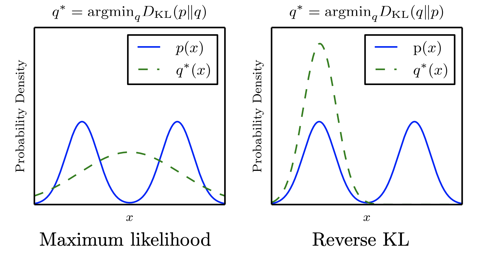
Unlike maximum likelihood, reverse KL tends to learn the mode. Here we show an example of a distribution over one-dimensional data $x$. In this example, we use a mixture of two Gaussians as the data distribution, and a single Gaussian as the model family. Because a single Gaussian can not capture the true data distribution, the choice of divergence determines the tradeoff that the model makes.

GAN problem

GAN is based on the zero-sum non-cooperative game. In short, if one wins the other loses. A zero-sum game is also called minimax. Your opponent wants to maximize its actions and your actions are to minimize them. In game theory, the GAN model converges when the discriminator and the generator reach a Nash equilibrium.

Since both sides want to undermine the others, a Nash equilibrium happens when one player will not change its action regardless of what the opponent may do. Consider two player $A$ and $B$ which control the value of $x$ and $y$ respectively. Player $A$ wants to maximize the value $xy$ while $B$ wants to minimize it.

\[\min_B\max_A V(A,B) = xy\]

The Nash equilibrium is $x=y=0$. We update the parameter $x$ and $y$ based on the gradient of the value function $V$.

Our example is an excellent showcase that some cost functions will not converge with gradient descent, in particular for a non-convex game.

It is possible that the Equation (1) cannot provide sufficient gradient for $G$ to learn well in practice. Generally speaking, $G$ is poor in early learning and samples are clearly different from the training data. Therefore, $D$ can reject the generated samples with high confidence. In this situation, $\log (1 − D (G (z)))$ saturates. I. Goodfellow et al. suggest to use the loss

\[J^{(G)} = \mathbb{E}_ {z \sim p(z)}[-\log(D(G(z)))] = \mathbb{E}_ {x \sim p_{gen}(x)}[-\log(D(x))].\]

In the minimax game, the generator minimizes the log-probability of the discriminator being correct. In this game, the generator maximizes the logprobability of the discriminator being mistaken. This new objective function results in the same fixed point of the dynamics of D and G but provides much larger gradients early in learning. However, the non-saturating game has other problems such as unstable numerical gradient for training $G$. With optimal $D^∗$, we have

\[\mathbb{E}_ {x \sim p_{gen}(x)}[-\log(D^* (x))] + \mathbb{E}_ {x \sim p_{gen}(x)}[\log(1 - D^* (x))] = D_{KL}(p_{gen}||p_{data}).\]

Recall that

\[\mathbb{E}_ {x \sim p_{data}(x)}[\log(D^* (x))] + \mathbb{E}_ {x \sim p_{gen}(x)}[\log(1 - D^* (x))] = 2D_{JS}(p_{gen}||p_{data}) - \log 4.\]

Therefore

\[\mathbb{E}_ {x \sim p_{gen}(x)}[-\log(D^* (x))] = D_{KL}(p_{gen}||p_{data}) - 2D_{JS}(p_{gen}||p_{data}) + \mathbb{E}_ {x \sim p_{data}(x)}[\log(D^* (x))] + \log 4.\]

We can see that the optimization of the alternative $G$ loss in the non-saturating game is contradictory because the first term aims to make the divergence between the generated distribution and the real distribution as small as possible while the second term aims to make the divergence between these two distributions as large as possible due to the negative sign. This will bring unstable numerical gradient for training $G$. Furthermore, KL divergence is not a symmetrical quantity, which is reflected from the following two examples: if $p_{data} \rightarrow 0$ and $p_{gen} \rightarrow 1$ we have $D_{KL}(p_{gen}||p_{data}) \rightarrow \infty$; if $p_{data} \rightarrow 1$ and $p_{gen} \rightarrow 0$ we have $D_{KL}(p_{gen}||p_{data}) \rightarrow 0$.

The penalizations for two errors made by $G$ are completely different. The first error is that $G$ produces implausible samples and the penalization is rather large. The second error is that $G$ does not produce real samples and the penalization is quite small. The first error is that the generated samples are inaccurate while the second error is that generated samples are not diverse enough. Based on this, $G$ prefers producing repeated but safe samples rather than taking risk to produce different but unsafe samples, which has the mode collapse problem.

There are many methods to approximate in GANs. Especially, we might like to be able to do maximum likelihood learning with GANs. Under the assumption that the discriminator is optimal, minimizing

\[J^{(G)} = \mathbb{E}_ {z\sim p_z}[-\exp(\sigma^{-1}(D(G(z))))]\]

where $\sigma$ is the logistic sigmoid function, is equavalent to minimize

\[D_{KL}(p_{data}||p_{gen}).\]

The proof is as follow, we wish to find a function $f$ such that the expected gradient of

\[J^{(G)} = \mathbb{E}_ {x\sim p_{gen}(x)}[f(x)]\]

is equal to the expected gradient of

\[D_{KL}(p_{data}||p_{gen}).\]

First we take the derivative of the KL divergence with respect to a parameter $\theta$

\[\frac{\partial}{\partial \theta} D_{KL}(p_{data}||p_{gen}) = - \mathbb{E}_ {x\sim p_{data}}\frac{\partial}{\partial \theta} \log p_{gen}(x).\]

We now want to find the $f$ that will make the derivatives of $J^{(G)}$ match above. We begin by taking the derivatives of $J^{(G)}$

\[\frac{\partial}{\partial \theta} J^{(G)} = \frac{\partial}{\partial \theta}\mathbb{E}_ {x \sim p_{gen}} f(x) = \int_x f(x) \frac{\partial}{\partial \theta} p_{gen}(x) = \int_x f(x) p_{gen}(x) \frac{\partial}{\partial \theta} \log p_{gen}(x)\]

where the last identity is by the derivative of $\log$, and we assume we can use Leibniz’s rule to exhange the order of differentiation and integration.

We see that the derivatives of $J^{(G)}$ come very near to giving us what we want; the only problem is that the expectation is computed by drawing samples from $p_{gen}$ when we would like it to be computed by drawing samples from $p_{data}$. We can fix this problem using an importance sampling trick; by setting $f = -\frac{p_{data}}{p_{gen}}$. Note that when constructing $J^{(G)}$ we must copy $p_{gen}$ into $f(x)$ so that $f(x)$ has a derivative of zero with respect to the parameters of $p_{gen}$. Fortunately, this happens naturally if we obtain the value of $\frac{p_{data}(x)}{p_{gen}(x)}$. Suppose our discriminator is given by $D(x) = \sigma(a(x))$ where $\sigma$ is the logistic sigmoid function. Suppose further that our discriminator has converged to its optimal value for the current generator,

\[D^* = \frac{p_{data}}{p_{data} + p_{gen}}.\]

Then $f(x) = − \exp (a(x))$.